ML Algorithm Explained: K Means Clustering
- By AIPI3 Machine Learning Team

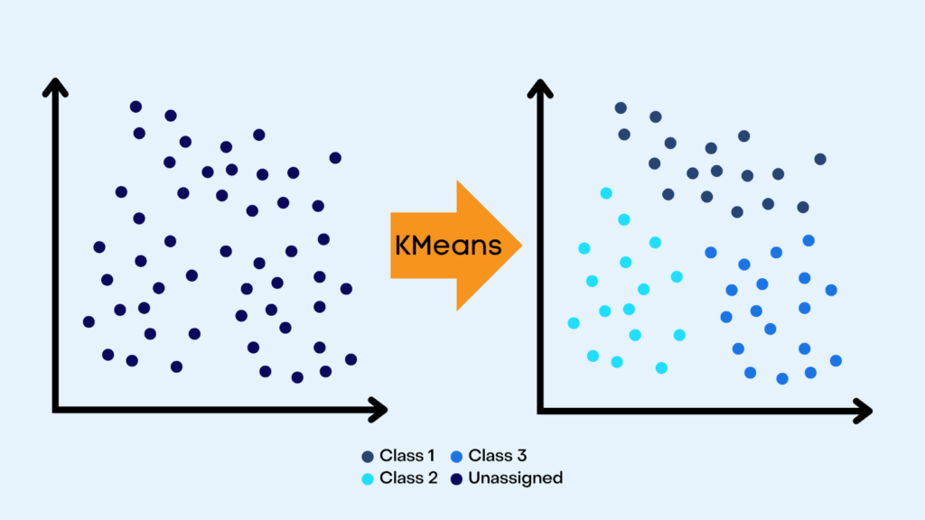
K Means Clustering is an unsupervised machine learning algorithm, that groups similar data points into “k” distinct clusters within a given data set. It is used for classification tasks. K Means has many applications such as customer segmentation, document clustering, anomaly detection, and much more.
Advantages:
- It is easy to implement due to its simplicity and ability to adapt to new data.
- It is highly scalable with large data sets.
Disadvantages:
- It is sensitive to outliers, mislabeled, and missing data.
- It is challenging to identify the right “k” value.
In this blog post, we provide an overview of the K Means
Clustering algorithm with an example of algorithm implementation with code.
Basic Concepts
KNN is a relatively simple algorithm with only two main parameters: a “k” value and a distance metric.

K-Value
The “k” value indicates the number of nearest data points that will be checked to determine the class of a given data point. For example, if “k” is set to 3, the algorithm checks the 3 closest points. The choice of “k” is dependent on the data under consideration but generally, it is recommended to have an odd “k” value to avoid ties.
Distance Metric
The distance metric is used to calculate the distance to the nearest point. While different decision measures can be chosen the most common is a Euclidean distance (Minkowski distance with p=2), which measures distance in a straight line between a given point and a neighboring point. The following formula is used to calculate this distance in a 2-dimensional space.

The distance between points is the sum of the square of the difference between the x and y coordinates of the points.
Algorithm Implementation with Code
Importing Libraries
For this example, we use scikit-learn, a popular machine learning library in python. Scikit-learn is a useful tool for creating datasets, training and testing algorithms, and much more. You must import all necessary libraries beforehand.
					import pandas as pd
import numpy as np

import matplotlib.pyplot as plt #plots
%matplotlib inline

from sklearn.datasets import make_blobs #synthetic dataset

from sklearn.cluster import KMeans #K Means Algorithm nd evaluations
Dataset
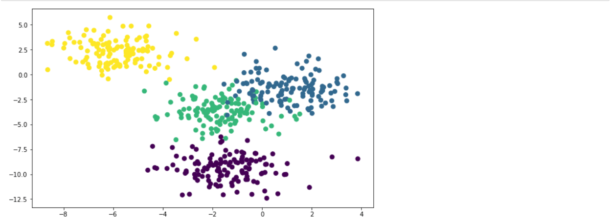
To create a synthetic dataset, we use make_blobs. The code below created a data set with 500 samples divided into 4 classes and 2 features.
					#create synthetic dataset
X, y = make_blobs(n_samples = 500, n_features = 2, centers = 4,
                       cluster_std = 1.5, random_state = 2)

#scatter plot of dataset
plt.figure(figsize = (10,6))
plt.scatter(X[:,0], X[:,1], c=y, marker= 'o', s=50)
plt.show()

The next step is to create a KMeans object, fit it to the training data and generate predictions based on the test data. As K means is an unsupervised algorithm, it is applied in instances where the initial clusters are unknown because it can identify patterns within a data set. Typically, the initial value of k is 2.
					kmeans = KMeans(n_clusters=2) #choosing k=2

kmeans.fit(X)

pred = kmeans.labels_
Evaluation
Finally, we evaluate the predictions by visually comparing the clusters in the original data with the clusters identified by the KMeans algorithm.
					f, (ax1, ax2) = plt.subplots(1, 2, sharey=True,figsize=(20,6))

ax1.set_title('KMeans Predictions')
ax1.scatter(X[:,0], X[:,1], c=pred, marker= 'o', s=50)

ax2.set_title('Original Data')
ax2.scatter(X[:,0], X[:,1], c=y, marker= 'o', s=50)

The resulting plot is quite different from the original clusters. For a K Means Clustering algorithm, the choice of K value is critical, therefore, we further check the algorithm performance against various K values by looking at the sum of squared distance (SSD) between data points and their assigned clusters’ centroids.
Choosing a K Value
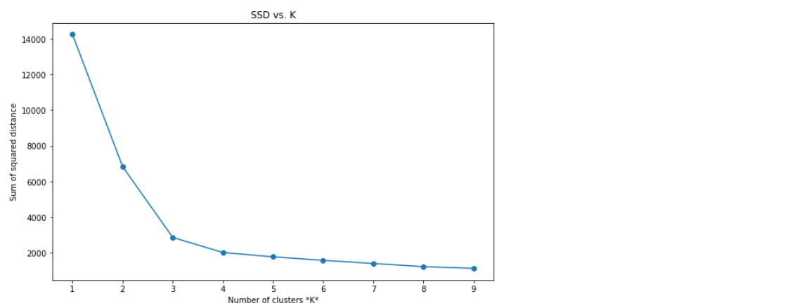
The code below calculates and compares the algorithm’s SSD against a range of K values and visualizes the results in a plot:
					ssd = [] #Sum of squared distance

for i in range(1,10):
    kmeans = KMeans(n_clusters=i)
    kmeans.fit(X)
    ssd.append(kmeans.inertia_)

plt.figure(figsize=(10, 6))
plt.plot(range(1,10), ssd, '-o')
plt.title('SSD vs. K')
plt.xlabel(r'Number of clusters *K*')
plt.ylabel('Sum of squared distance');

Here we can see that after around K=4 onwards, the SSD begins to flatten out and form an elbow. We can further confirm if this is a good k-value by visually comparing the clusters.
					kmeans = KMeans(n_clusters=4)

kmeans.fit(X)

pred = kmeans.labels_

f, (ax1, ax2) = plt.subplots(1, 2, sharey=True,figsize=(20,6))

ax1.set_title('KMeans Predictions with K=4')
ax1.scatter(X[:,0], X[:,1], c=pred, marker= 'o', s=50)

ax2.set_title('Original Data')
ax2.scatter(X[:,0], X[:,1], c=y, marker= 'o', s=50)

The resulting plot does a reasonable job of predicting the clusters within the dataset. In business applications, you would use datasets generated from various business processes. However, the basic process of using the algorithm remains the same.
Tags: Unsupervised, Clustering, Parametric, NP-Hard, Heuristic Convergence, Local Minimum
AIPI3’s ML platform uses many innovative machine learning algorithms to create value for businesses. Our platform is driven by artificial intelligence & machine learning experts with extensive experience across a wide range of industries, specializations, and applications.
Get in touch with AIPI3 to discover how we can assist you!
