ML Algorithm Explained: Linear Regression
- By AIPI3 Machine Learning Team

Linear Regression is a supervised machine learning algorithm, which predicts the value of a given data point based on the values of independent variables. It is used for regression tasks. Different linear regression models are applicable based on the relationships between dependent and independent variables and the number of variables under consideration. Linear Regression has many applications such as financial predictions, sales forecasting, price estimation, and much more.
Advantages:
- It is easy to implement and interpret compared to other algorithms.
- It can extrapolate values beyond the given dataset.
- It can handle overfitting well using dimensional reduction, regularization, and cross-validation.
Disadvantages:
- It assumes a linear relationship between dependent and independent variables.
- It is susceptible to noise and outliers.
In this blog post, we provide an overview of the Linear Regression algorithm with an example of algorithm implementation with code.
Basic Concepts
Linear regression predicts the value of a dependent variable y based on an independent variable X. In its simplest form we use a single value of x to predict y, which can be represented as follows:

Where:
- y represents the actual value of y
- (a0 + a1x) represents the predicted value of y
- a0 represents the y-intercept
- a1 represents the coefficient
Cost Function
The goal of linear regression is to achieve the best-fit regression line and minimize the error between the predicted value of y and the actual value of y. There are three common types of errors that are relevant to regression problems:
Mean Absolute Error (MAE) is the mean of the absolute value of the difference between predicted y and actual y:

Root Mean Squared Error (RMSE), is the square root of the mean of the squared difference between predicted y and actual y:

Root Mean Squared Error (RMSE), is the square root of the mean of the squared difference between predicted y and actual y:

All of these are Cost Functions (J), which we are looking to minimize. However, generally we are interested in minimizing the RMSE in linear regression:

Gradient Descent
Gradient descent is a method of updating a0 and a1 to minimize the cost function. By starting at random values of a0 and a1, we iteratively alter these values until the minimum cost is achieved.
Algorithm Implementation with Code
Importing Libraries
For this example, we use scikit-learn, a popular machine learning library in python. Scikit-learn is a useful tool for creating datasets, training and testing algorithms, and much more. You must import all necessary libraries beforehand.
					import pandas as pd
import numpy as np

import matplotlib.pyplot as plt #plots
%matplotlib inline

from sklearn.datasets import load_diabetes #dataset
from sklearn.model_selection import train_test_split #Splitting the data into testing and training data sets

from sklearn.linear_model import LinearRegression #Linear Regression Algorithm
Dataset
To create the dataset, we use load_diabetes. The diabetes dataset is a popular dataset used in machine learning. This dataset contains data from diabetic patients and contains ten variables such as their BMI, age, blood pressure, glucose levels, etc.
					# load the diabetes dataset
diabetes = load_diabetes()

db = pd.DataFrame(diabetes.data, columns = diabetes.feature_names) #variables that influence risk of diabetes
db['target'] = diabetes.target #target variable that predicts risk of diabetes

# store the feature matrix (X) and response vector (y)
X = db.drop(labels='target', axis=1) #All variables except the target variable
y = db['target']
Test Train Split
In this section, we split the dataset into training data and testing data. The objective is to train the algorithm to predict a value of y based on its associated X values. This allows us to test the performance of the algorithm against testing data by comparing the predicted values with the actual value.
X_train, X_test, y_train, y_test = train_test_split(X, y, test_size=0.25, random_state=101)
The next step is to create a Linear Regression object, fit it to the training data and generate predictions based on the test data.
					lm = LinearRegression()

lm.fit(X_train,y_train)

pred = lm.predict(X_test)
Evaluation
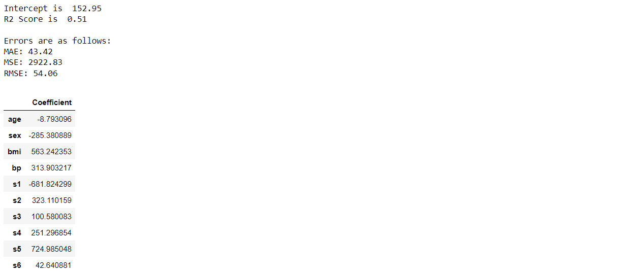
Finally, we evaluate the predictions using the intercept, coefficient, error, and r-2 values, which are used to measure the performance of the regression algorithm.
					#Intercept
print("Intercept is ", round(lm.intercept_,2))

#@2 score
print("R2 Score is ", metrics.r2_score(y_test,pred).round(2))

#Error
print('\nErrors are as follows:')
print('MAE:', metrics.mean_absolute_error(y_test, pred).round(2))
print('MSE:', metrics.mean_squared_error(y_test, pred).round(2))
print('RMSE:', np.sqrt(metrics.mean_squared_error(y_test, pred)).round(2))

#Coefficient
coeff_df = pd.DataFrame(lm.coef_,X.columns,columns=['Coefficient'])
coeff_df

In business applications, you would use datasets generated from various business processes. However, the basic process of using the algorithm remains the same.
Tags: Supervised, Linear, Parametric, Close-Form, Non-Linear Mapping, Kernel Trick
AIPI3’s ML platform uses many innovative machine learning algorithms to create value for businesses. Our platform is driven by artificial intelligence & machine learning experts with extensive experience across a wide range of industries, specializations, and applications.
Get in touch with AIPI3 to discover how we can assist you!
